Two portfolio management case studies

These are the two case studies I wrote for Applied Portfolio Management, ECFS 843, one of the ten subjects in Macquarie University’s Master of Applied Finance. They are undated; the major assignment for the same subject was due on the 4th of June 1993, which is the date used here. The title is mine — the manuscript is headed only “Case Studies”.

The organisation chart is the one embedded in the manuscript, recovered from the metafile Word cached for it and converted to vector rather than reproduced as a screenshot. It is my redrawing of the chart in the case, not artwork from the case itself.

Set from the Word 2.0 manuscript, and the answers are as submitted.

Download the original case studies (DOC, 38 KB)

Master of Applied Finance

ECFS 843: Applied Portfolio Management

Case Studies

Chris Tham

SID 30957109

Case Study: The Common Fund

What is the Common Fund?

The Common Fund is a non profit corporation owned, organised and operated by and for its members, which are educational institutions. It provides investment management services for its members in the context of endowment, quasi-endowment and operating funds. It does this by operating several pooled funds managed by a selection of investment management organisations. It also conducts a program of research and publication related to the fiscal management of educational institutions.

How does the TSA Asset Allocation scheme work?

The asset allocation scheme works by monitoring on a daily basis the following rates, corresponding to three asset classes (cash, bonds and equities):

• short term interest rates

• 20 year US Treasury bonds

• earnings yield on the S&P 500 Stock Index, which are “normalised” by performing a regression analysis on the earnings for the past 16 quarters which is then divided by the current price of the index.

The scheme then compares the relative returns of the different asset classes against their historical or “normal” long term equilibrium relationships. This involves calculating the return spreads between the classes and comparing the spreads against risk premium relationships obtained from historical data.

It also looks at the following factors which influence bond and equity returns:

1. US economic growth

2. level and direction of real short term rates

3. price momentum in bonds and equity

4. price volatility in bonds and equity

By combining the relative return comparisons and the above factors, a specific measure of the relative attractiveness of the various asset classes is calculated each day, together with an optimal mix of the asset classes that will generate the highest expected return.

As markets fluctuate, the relative attractiveness of each asset class changes. The scheme attempts to increase the return of the fund by shifting the asset mix of the fund whenever the change is deemed to be sufficiently large to make the shift profitable (the minimum move is usually a 5% shift). This is done by increasing exposure to asset classes with higher potential relative returns and decreasing exposure to asset classes with lower potential relative returns. Usually, between one to three shifts are made every fortnight.

Since the shifts attempt to anticipate changes in asset class valuations, the scheme is contrairian in nature, by investing in asset classes containing a high “risk premium” for which the market consensus is bearish.

The benchmark for the scheme, also called the “neutral” portfolio, is the relative participation of each investor in the Common Fund’s equity and fixed income pools.

The scheme uses equity index and bond futures to effect shifts in asset allocation rather than direct trading in and out of the asset classes, in order to minimise transaction costs and decreasing to time required to implement the shift.

Compare the risks of AA with a “buy and hold” policy.

Sharpe¹ made the following points in comparing between an asset allocation scheme and a “buy and hold” policy:

• In an efficient market, it will be difficult to be able to identify changes in relative returns between asset classes and without superior predictive ability, the asset allocator is likely to forego return by shifting from equity to cash.

• Shifting from one asset class to another entail non-recoverable transaction costs.

• AA exposes the fund to larger losses when errors are made.

Sharpe then formulated a model comparing a simple “market timing” strategy against a “buy and hold” strategy over three different periods and made the following conclusions:

1. The difference in returns between “perfect” timing and holding equity exclusively is only around 4.5% p.a. and the difference between “perfect” timing and holding a constant asset mix with the same variability is around 6.5%.

2. Historically, the proportion of periods in which the equity return was higher than the cash return is 0.60-0.70. Hence, an AA strategist must be able to predict correctly when to shift the asset mix more often than this or risk performing worse than the equity index.

3. It is likely that return assumptions may change over time.

Jeffrey² made the following observations:

• Empirical research generally have failed to detect any market timing skills among professional investors.

• The potential loss from market timing is twice as large as the potential gain.

• Most positive returns from investing in equity is “compressed” in just a few periods, hence by shifting investment from one asset class to another, the fund risks the danger of “missing out” on some or all of those periods.

• The chances of making correct asset shift decisions in the absence of superior knowledge become slimmer as the time frame of the strategy increases and also as the frequency of the timing interval increases.

These views are opposed by Wilson Sy³, who offer the following counter-arguments:

• Markets are not necessarily efficient, at least in the strong form and it is possible to acquire private or “insider” information.

• It may be difficult to measure the performance of market timing activities without additional information not generally available to researchers.

• The use of derivatives in making asset switches can result in low transaction costs.

• Over the years, cash rates have become higher and the proportion of periods in which equity return does not dominate cash return has become higher, so the penalty for mistiming has become less severe and a successful market timer need not have as high a predictive accuracy as Sharpe suggests.

• Avoiding losses in equity markets have become more important than missing out on a period in which the equity return was exemplary.

• The potential gain (and loss) from market timing is higher as the frequency of timing interval increases.

• The level of predictive accuracy required to break even also decreases slightly with the frequency of portfolio revision.

• The volatility of returns from market timing is less than the equity volatility, but the portfolio weights will become more volatile.

In the context of the TSA AA scheme, the following comments can be made:

• The frequency of portfolio revision is fairly high, around one-three times a fortnight, hence increasing the potential gain (and risks) from market timing.

• The strategy for determining the optimal asset mix is analogous to the strategy of buying undervalued stocks (as measured by a low Price-Earnings ratio) and selling overvalued stocks. There are some empirical evidence supporting the effectiveness of the latter strategy.

• Recent empirical research has casts some doubts over the efficiency of bond and equity markets. This may “explain” why the strategy may succeed.

• The risks from the AA strategy are:

1. Moving into an asset mix which upon reflection may be sub optimal may result in foregone returns, or, in some cases, actual losses.

2. Using the futures market results in a basis risk when the futures market moves differently from that of the underlying assets.

3. The futures market may be mispriced due to supply/demand factors.

4. The underlying risk premium relationships may change over time.

5. Trading in equity index futures is not a perfect substitute for trading in the underlying equity assets (risk, expected return, dividend yield). For example, an underlying equity asset class generates dividend returns, and futures positions generate margin calls.

How sound is the theoretical basis of this version of AA?

• The AA scheme assumes that the historical risk premium equilibrium relationships will hold over time, or does not depend on factors other than those used by the asset allocation model.

• Like any theoretical model, the accuracy of its results depend on the accuracy of its inputs, which in this case include normalised equity yields and forecasts of other factors.

• It also implicitly assumes that the markets for the various asset classes are not strictly efficient, otherwise the strategy will not be able to generate positive returns over and above a buy and hold strategy.

• Different strategic asset allocation models sometimes produce dramatically different results, which is disturbing.

• There are some issues arising from the use of futures to effect shifts in asset allocation (see above).

In summary, the strategy is attempting to infer future return behaviour from past relationships and current trends and capitalising on this inference by shifting the asset mix of the fund. Whether this is objectionable or not depends on whether one is a believer or otherwise of the theory of efficient markets.

Would you recommend it to your clients?

Maybe.

Case Study: Sanford C Bernstein & Co, Inc

What are the driving forces in Bernstein & Co?

Sanford C. Bernstein & Co., was an investment management firm serving both private individuals and corporate and public pension funds. The firm was also in the business of selling institutional research and brokerage services. The firm was started by Sanford C. Bernstein (now Zalman Bernstein) in 1967 to manage the money of private individuals. The philosophy of the firm was that high quality value oriented research was the key to producing superior returns.

By 1979, the firm had entered into the market for institutional research and was delivering a product based upon the detailed analysis of a company, driven by a long run forecast of future macro-economic, sector specific and industry specific variables, performed from the point of view of the long term oriented corporate planner.

At about the same time, the money management operations were expanded to include pension funds. The firm also decided to adopt a methodology for the investment process that was disciplined and systematic, linked directly to the company’s research. They eventually decided upon a methodology using the dividend discount model.

The following differentiates Bernstein & Co. from other money managers:

• The firm’s belief and commitment to its investment philosophy.

• The firm’s ability to handle dramatic expansion and yet continue to work with private investors.

• The firm’s investment in its computer capability and investment management systems.

• The firm’s reliance on the dividend discount model with total consistency.

• The firm contrairian stance as a value investor.

In summary, the driving force of the firm is basically its systematic investment approach, combined with its adherence to fundamental research.

How is Bernstein & Co organised?

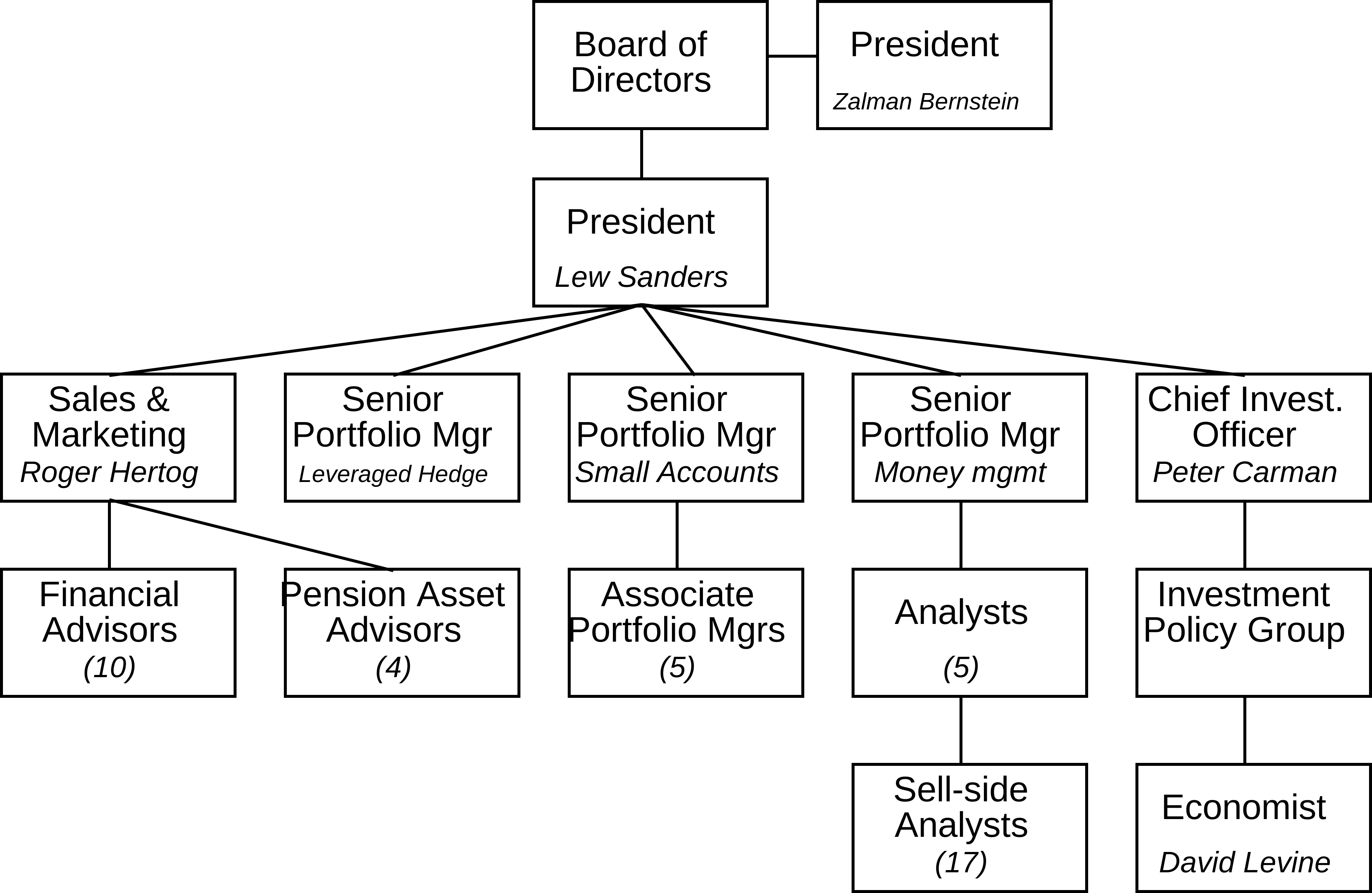
The following chart describes the organisation of the money management operations in 1983.

µ §

Associate Portfolio Managers were college graduates with no prior experience in portfolio management. They did not have any client contact.

Financial Advisors obtained accounts and counsel the clients on objective setting, risk level selection, investment goals, tax implications, and available investment techniques.

The Pension Asset Advisors establish the initial relationship, obtain the account and coordinate the firm’s relationship with the pension clients.

The Senior Portfolio Managers took an active part in presentations to new accounts and met with existing clients on a semi-annual basis.

Small accounts were managed by one Associate Portfolio Managers under the guidance of one Senior Portfolio Manager. The equity portions of the balanced accounts were managed together with other large equity accounts by four of five Senior Portfolio Managers (this includes Peter Carman and Lew Sanders). The fifth Senior Portfolio Manager ran the Leveraged Hedge specialty product.

All investment decisions were made by the Investment Policy group consisting of Zalman Bernstein, Lew Sanders, the firm’s economist and the remaining Senior Portfolio Managers.

Other divisions mentioned in the Institutional Investment article:

• Investment Management Systems

• Fixed income mutual fund group, involved in fixed income investments and fixed income research.

What is Bernstein’s system of stock selection?

Bernstein’s system of stock selection is based on the dividend discount model. Working within an investment universe of about 500 stocks that corresponded approximately to the S&P 500, the internal rate of returns of these securities were computed as the discount rate that equated the present value of Bernstein’s own estimates of each company’s stream of future expected dividend payments to the company’s current stock price.

The stream of future dividends is estimated by building a model for each company that related its future dividend payments to a forecast of its future profitability and growth in earnings. The future is segmented into three time periods:

1. An initial five year phase, in which the earnings and dividend estimates of the Bernstein analysts were used, or obtained from reputable outside analysts if the company was not followed by a Bernstein analyst.

2. A transition phase, which is a period of time taken by the company to make the transition from its forecast profitability and growth rates in the initial period to the terminal phase. The number of years and the manner of the transition phase varied from company to company to reflect the growth path of the company.

3. The terminal phase went on into perpetuity. All companies were assumed to have constant growth rates and payout ratios during this phase. Two different sets of numerical values were used for all companies (the choice of which set was appropriate depended on whether the company were classified as a utility), based on long run historical averages adjusted to reflect Bernstein’s own long run forecast for growth, inflation and profitability in the economy as a whole.

The stock selection process was based on investor psychology causing individual companies as well as whole sectors of the economy to be undervalued with respect to other companies/sectors. Accordingly, the firm utilises active sector allocation as well as stock selection within the sectors.

What types of stocks does it throw up as “buys” and “sells”?

The stock selection process favours stocks with high internal rates of return, or, in the jargon of value investors, “undervalued” stocks. This would be stocks that would usually have low Price-Earnings ratios and would be classified as “value” stocks. Stocks with very low internal rates of return would be candidates for sells. These stocks would usually be perceived by the market as “growth” stocks having high Price-Earnings ratios.

In fact, the firm has a strict selling discipline: stocks could only be sold if they were not ranked in the top quintile. Furthermore, they had to be sold if they were ranked in the middle of the third quintile or lower (lower 50% of the universe).⁴

How does Bernstein form portfolios?

The Investment Policy group selects five model investment portfolios from the top quintile of the internal rate of return rankings (i.e. the 20% of companies with the highest internal rates of return). These model portfolios serve as “templates” for the various equity accounts and correspond to the five risk categories which were differentiated by diversification requirements. Each account was preassigned to a risk category and was to be matched as closely as possible to the model portfolio of that category, subject to the firm’s sell disciplines and account specific factors such as tax consequences and restrictions regarding the purchase of particular stocks.

The model portfolios are formed by considering the representation of each sector in the top quintile. A commitment was made to a particular sector if many companies within the sector appeared in the top quintile. Hence the weighting of the sectors in the model portfolios would be closely related to their weighting in the top quintile. Sectors with only a few stocks in the top quintile would usually be omitted, and the weights of the remaining sectors adjusted to take into account the fact that the investment universe was not equally distributed across sectors.

An initial candidate list of around 60 stocks for the model portfolios would then be formed from the most highly ranked companies in each of the chosen sectors. Basing on the firm’s confidence in each company’s earnings estimates and assessment of the likelihood of earnings surprise, as well as the sensitivity of the company’s position in the rankings to changes in these estimates, would narrow down the list to about 35-45 stocks per portfolio.

What dimension of tracking error might you expect from Bernstein’s approach?

In the paper by David Begg⁵, he considered the performance of an actively managed fund in relation to a static benchmark portfolio and introduced the concept of the Active or Swing Portfolio, which is the differences in the individual sector allocations between the current portfolio and the benchmark portfolio. Tracking error, which is a measure of the relative risk of the current and benchmark portfolios, is then defined to be the standard deviation of return on the swing portfolio, which is equal to the standard deviation of the expected return differential between the two portfolios. The two dimensions of tracking error in a portfolio come from differences arising from:

1. asset allocation between the permitted asset sectors, and

2. stock selection within each individual sector to outperform the sector target.

In the context of Bernstein’s approach, given that Bernstein did not actively vary the asset mix of the balanced accounts, the tracking error of the model portfolios against their individual benchmark portfolios would arise solely from stock selection risk.

However, if we ignore the fixed income portions of the balanced accounts, then the relevant benchmark portfolio against the equity accounts (or the equity component of the accounts) would be the S&P 500. In the context of Bernstein’s equity portfolios, the tracking error would arise from both sector allocation risk (with the sectors being defined as sectors of the economy rather than different asset classes) and stock selection risk within each sectors. This is understandable as the dividend discount model is used for active sector allocation as well as stock selection within the sectors.

Conclusion

The performance of the Bernstein approach is sensitive to:

1. errors in the general economic outlook forecast, as well as

2. the accuracy of the relative growth rates and earnings estimates among companies.

The model seems to be based on the premise that the market has at times exhibited a willingness to discount growth rates in dividends which are much different from average, for prolonged periods of time, into the current prices of equity. The true growth horizon, which is the length of time into the future that a typical investor can actually predict with some degree of confidence that a given firm’s earnings will grow faster or slower than average, is relatively short (4-5 years) but the market perceives the growth horizon to be much longer.

This is a form of market inefficiency which causes a distortion of the relationship between risk and return and empirical evidence shows that stocks with poorer than average growth prospects (“value” stocks) will outperform stocks with strong growth prospects (“growth” stocks) and studies have shown that firms with histories of relatively fast growth rates fail to keep up the pace.

As a result, value stocks tend to be undervalued and growth stocks tend to be overvalued. The Bernstein approach throws up value stocks as “buys” and growth stocks as “sells” in order to profit from this form of market inefficiency. This strategy will work as long as the market exaggerate the length of time for which they can forecast relative growth and a subsequent correction occurs. However, during periods when investors are in the process of extending the perceived growth horizons, perhaps because few growth surprises are expected, then growth stocks will outperform value stocks. This in fact happened during the period 1989-1991.

Chris Tham ECFS 843: Applied Portfolio Management Page 9

Notes

1. William F Sharpe, Likely Gains from Market Timing, Financial Analysts Journal, March-April 1975.
2. Robert H Jeffrey, The folly of stock market timing, Harvard Business Review, July-August 1984.
3. Wilson Sy, Market timing: Is it a folly?, The Journal of Portfolio Management, Summer 1990.
4. The Institutional Investor article implies that by 1989 this selling rule has been modified to the bottom 40% of stocks.
5. David A Begg, Portfolio Control: Risk and Performance